7.1 Building an interaction
library(rethinking)
data(rugged)
d <- rugged
How does terrain ruggedness influence the GDP?
# make log version of outcome
d$log_gdp <- log(d$rgdppc_2000)

dd <- d[ complete.cases(d$rgdppc_2000), ]

# split into Africa andnot-Africa
d.A1 <- dd[ dd$cont_africa == 1, ]
d.A0 <- dd[ dd$cont_africa == 0, ]
Make two model: one for Africa, one for non-Africa:
# Africa
m7.1 <- map(
  alist(
    log_gdp ~ dnorm( mu, sigma) ,
    mu <- a + bR*rugged ,
    a ~ dnorm(8, 100),
    bR ~ dnorm( 0, 1 ),
    sigma ~ dunif( 0, 10 )
  ), data=d.A1
)

# non-Africa
m7.2 <- map(
  alist(
    log_gdp ~ dnorm( mu, sigma ),
    mu <- a + bR*rugged ,
    a ~ dnorm( 8, 100),
    bR ~ dnorm( 0, 1),
    sigma ~ dunif( 0, 10 )
  ), data=d.A0
)
Make some plots:
rug.seq <- seq(from=-1, to=8, length.out = 30)
africa.mu <- link( m7.1, data=data.frame(rugged=rug.seq) )
africa.mu.mean <- apply(africa.mu, 2, mean)
africa.mu.PI <- apply(africa.mu, 2, PI)

non.africa.mu <- link( m7.2, data=data.frame(rugged=rug.seq))
non.africa.mu.mean <- apply(non.africa.mu, 2, mean)
non.africa.mu.PI <- apply(non.africa.mu, 2, PI)

par(mfrow=c(1,2))
plot( log_gdp ~ rugged, data=d.A1, col="steelblue")
lines(rug.seq, africa.mu.mean)
shade(africa.mu.PI, rug.seq)
mtext("Africa")

plot( log_gdp ~ rugged, data=d.A0, col="black")
lines(rug.seq, non.africa.mu.mean)
shade(non.africa.mu.PI, rug.seq)
mtext("not Africa")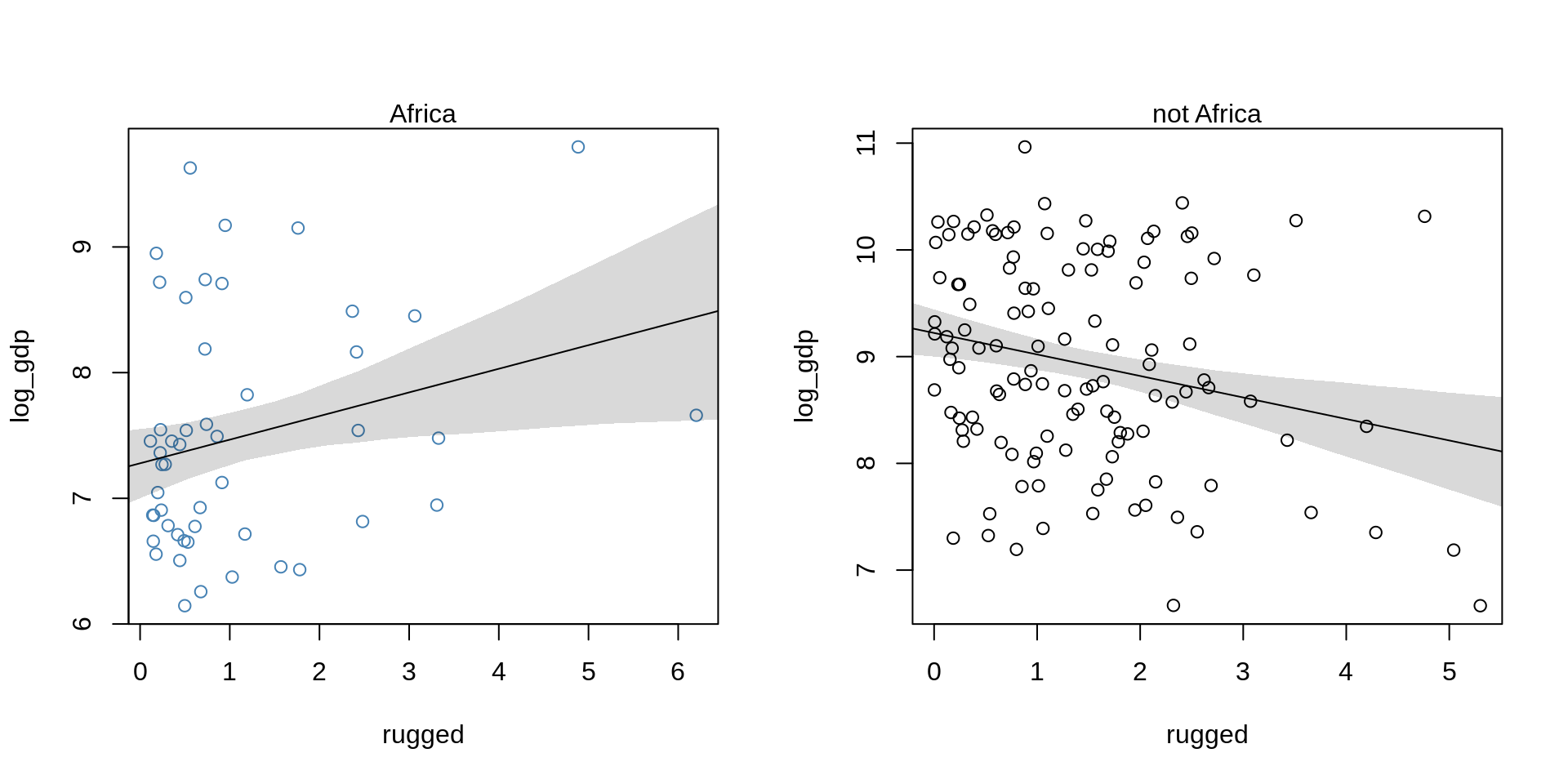
Ruggedness seems to have different influence for countries outside and inside Africa, the slope is actually reversed! How can we capture the reversed slopes in a single model using all data?
A simple regression on all the data:
m7.3 <- map(
  alist(
    log_gdp ~ dnorm( mu, sigma),
    mu <- a + bR*rugged,
    a ~ dnorm( 8, 100),
    bR ~ dnorm(0, 1) ,
    sigma ~ dunif( 0, 10)
  ), data=dd
)
A regression with a dummy variable for African nations:
m7.4 <- map(
  alist(
    log_gdp ~ dnorm( mu, sigma ),
    mu <- a + bR*rugged + bA*cont_africa,
    a ~ dnorm( 8, 100),
    bR ~dnorm( 0, 1),
    bA ~ dnorm( 0, 1),
    sigma ~ dunif(0, 19)
  ), data=dd
)
Compare the two models:
compare( m7.3, m7.4)## WAIC SE dWAIC dSE pWAIC weight
## m7.4 476.4369 15.30824 0.0000 NA 4.430565 1.000000e+00
## m7.3 539.6087 13.26703 63.1718 15.05826 2.704404 1.916095e-14plot( compare( m7.3, m7.4 ))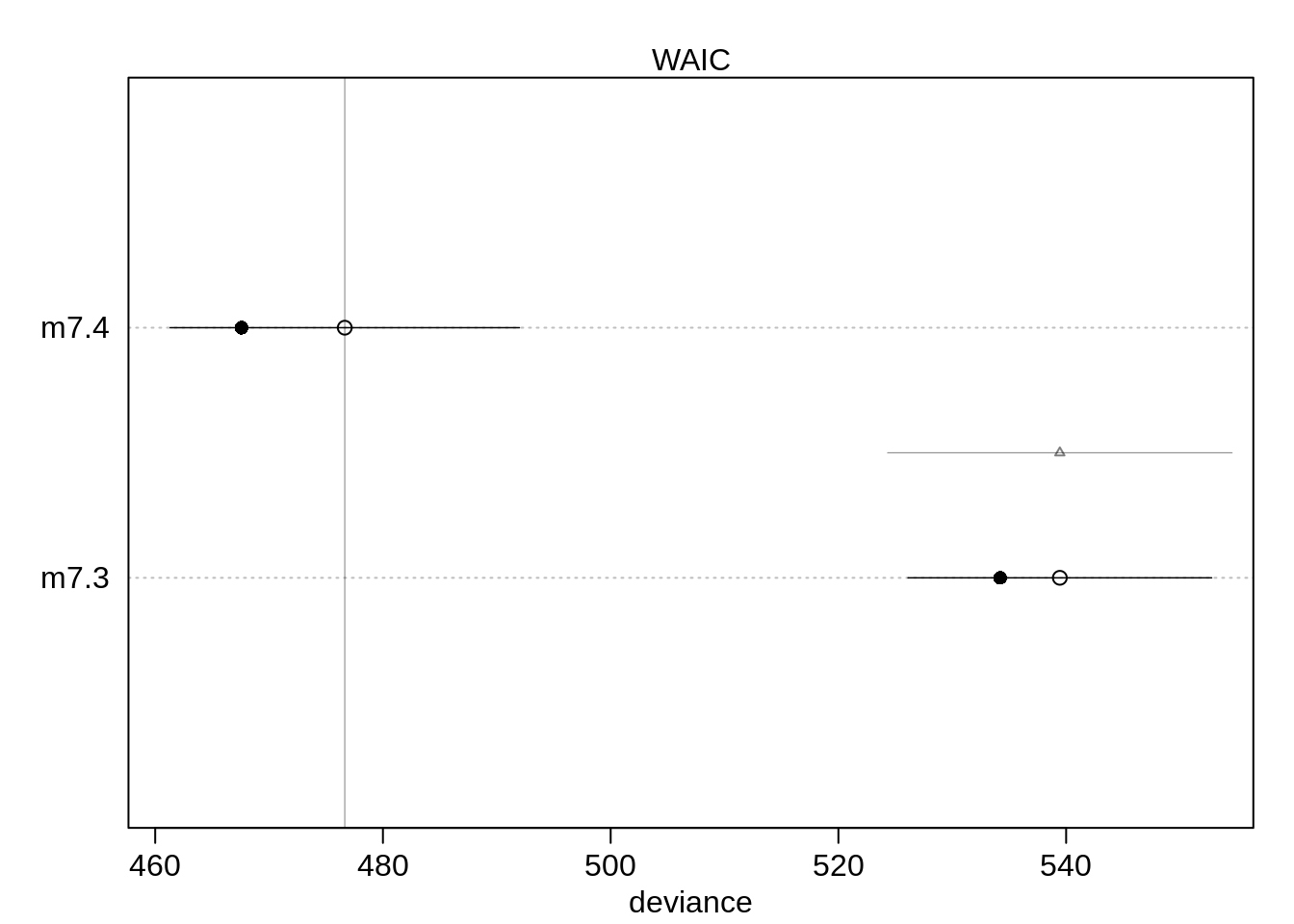
The model with the dummy-variable does perform better than without. Let’s plot the dummy-variable model.
# mu, fixing cont_africa=0
mu.NotAfrica <- link( m7.4, data=data.frame(rugged=rug.seq, cont_africa=0 ) )
mu.NotAfrica.mean <- apply(mu.NotAfrica, 2, mean )
mu.NotAfrica.PI <- apply(mu.NotAfrica, 2, PI)

# mu, fixing cont_africa=1
mu.Africa <- link( m7.4, data=data.frame(rugged=rug.seq, cont_africa=1 ) )
mu.Africa.mean <- apply( mu.Africa, 2, mean )
mu.Africa.PI <- apply( mu.Africa, 2, PI )

plot( log_gdp ~ rugged, data=d.A1, col="steelblue",
      xlab="Terrain Ruggedness Index",
      ylim= range(dd$log_gdp))
points( log_gdp ~ rugged, data=d.A0, col="black")

lines(rug.seq, mu.Africa.mean, col="steelblue")
shade(mu.Africa.PI, rug.seq, col=col.alpha("steelblue"))
text(4, 6.8, "Africa", col="steelblue")

lines(rug.seq, mu.NotAfrica.mean, col="black")
shade(mu.NotAfrica.PI, rug.seq, col=col.alpha("black"))
text(4.5, 9.25, "not Africa")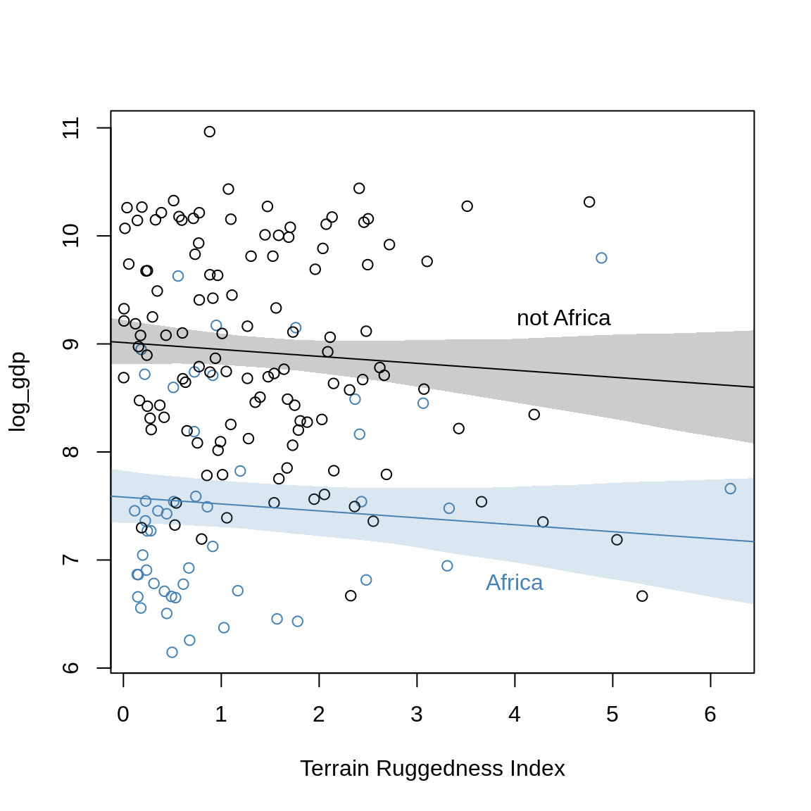
The dummy-variable has only moved the intercept.
Adding an interaction
m7.5 <- map(
  alist(
    log_gdp ~ dnorm(mu, sigma),
    mu <- a + gamma*rugged + bA*cont_africa,
    gamma <-bR + bAR*cont_africa,
    a ~ dnorm( 8, 100),
    bA ~ dnorm(0, 1),
    bR ~ dnorm(0, 1),
    bAR ~ dnorm( 0, 1),
    sigma ~ dunif( 0, 10)
  ), data=dd
)

compare( m7.3, m7.4, m7.5 )
## WAIC SE dWAIC dSE pWAIC weight
## m7.5 469.9787 15.19990 0.000000 NA 5.507534 9.625579e-01
## m7.4 476.4723 15.38920 6.493594 6.33570 4.441759 3.744215e-02
## m7.3 539.5198 13.18796 69.541095 15.20289 2.672832 7.634312e-16plot( compare( m7.3, m7.4, m7.5))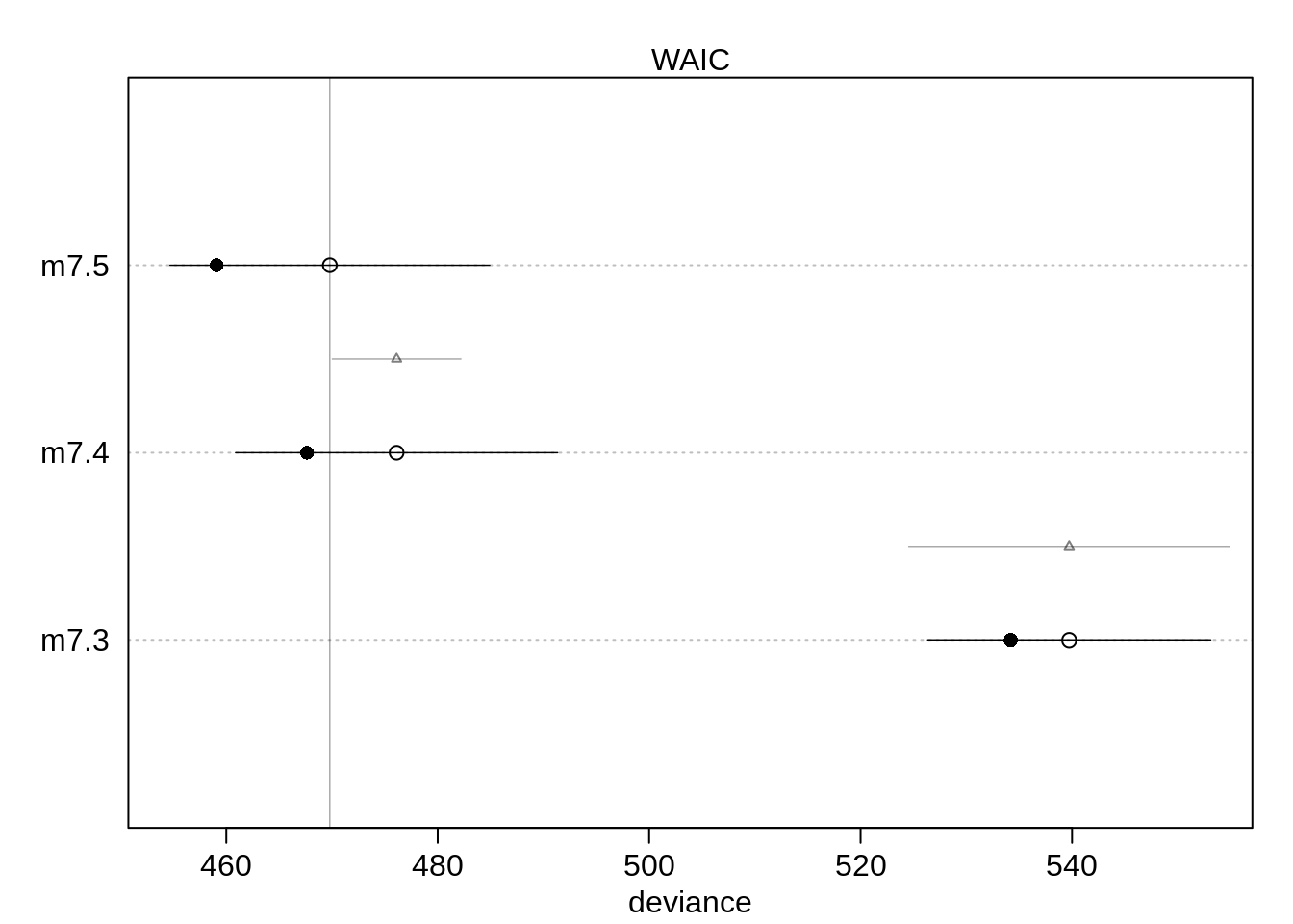
The interaction model performs better than the other two, though it only performs slightly better than the dummy variable: Since there are few countries in Africa, the data are sparse.
Plotting interactions
mu.Africa <- link( m7.5, data=data.frame(cont_africa=1, rugged=rug.seq))
mu.Africa.mean <- apply(mu.Africa, 2, mean)
## Error in apply(mu.Africa, 2, mean): dim(X) must have a positive lengthmu.Africa.PI <- apply(mu.Africa, 2, PI)## Error in apply(mu.Africa, 2, PI): dim(X) must have a positive lengthmu.NotAfrica <- link( m7.5, data=data.frame(cont_africa=0, rugged=rug.seq))
mu.NotAfrica.mean <- apply(mu.NotAfrica, 2, mean)## Error in apply(mu.NotAfrica, 2, mean): dim(X) must have a positive lengthmu.NotAfrica.PI <- apply(mu.NotAfrica, 2, PI )## Error in apply(mu.NotAfrica, 2, PI): dim(X) must have a positive lengthpar(mfrow=c(1,2))
plot( log_gdp ~ rugged, data=d.A1,
col="steelblue", ylab="log GDP year 2000",
xlab="Terrain Ruggedness Index")
mtext("African nations")
lines(rug.seq, mu.Africa.mean, col="steelblue")
shade( mu.Africa.PI, rug.seq, col=col.alpha("steelblue"))
plot( log_gdp ~ rugged, data=d.A0,
col="black", ylab="log GDP year 2000",
xlab="Terrain Rugggedness Index")
mtext( "Non-African nations", 3)
lines( rug.seq, mu.NotAfrica.mean )
shade( mu.NotAfrica.PI, rug.seq )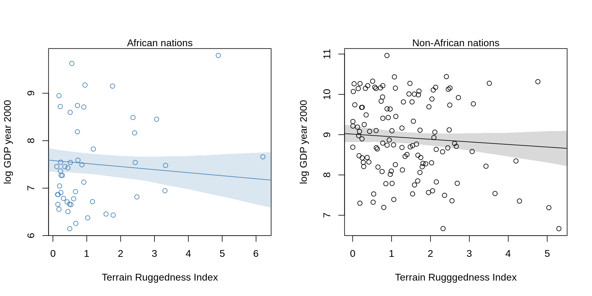
The slope reverses! We can also overlap the plots:
plot( log_gdp ~ rugged, data=d.A1, col="steelblue",
      xlab="Terrain Ruggedness Index",
      ylim=range(dd$log_gdp))
points( log_gdp ~ rugged, data=d.A0, col="black")

lines(rug.seq, mu.Africa.mean, col="steelblue")
shade( mu.Africa.PI, rug.seq, col=col.alpha("steelblue"))
text(4, 6.8, "Africa", col="steelblue")

lines( rug.seq, mu.NotAfrica.mean )
shade( mu.NotAfrica.PI, rug.seq )
text(4.5, 9.25, "not Africa")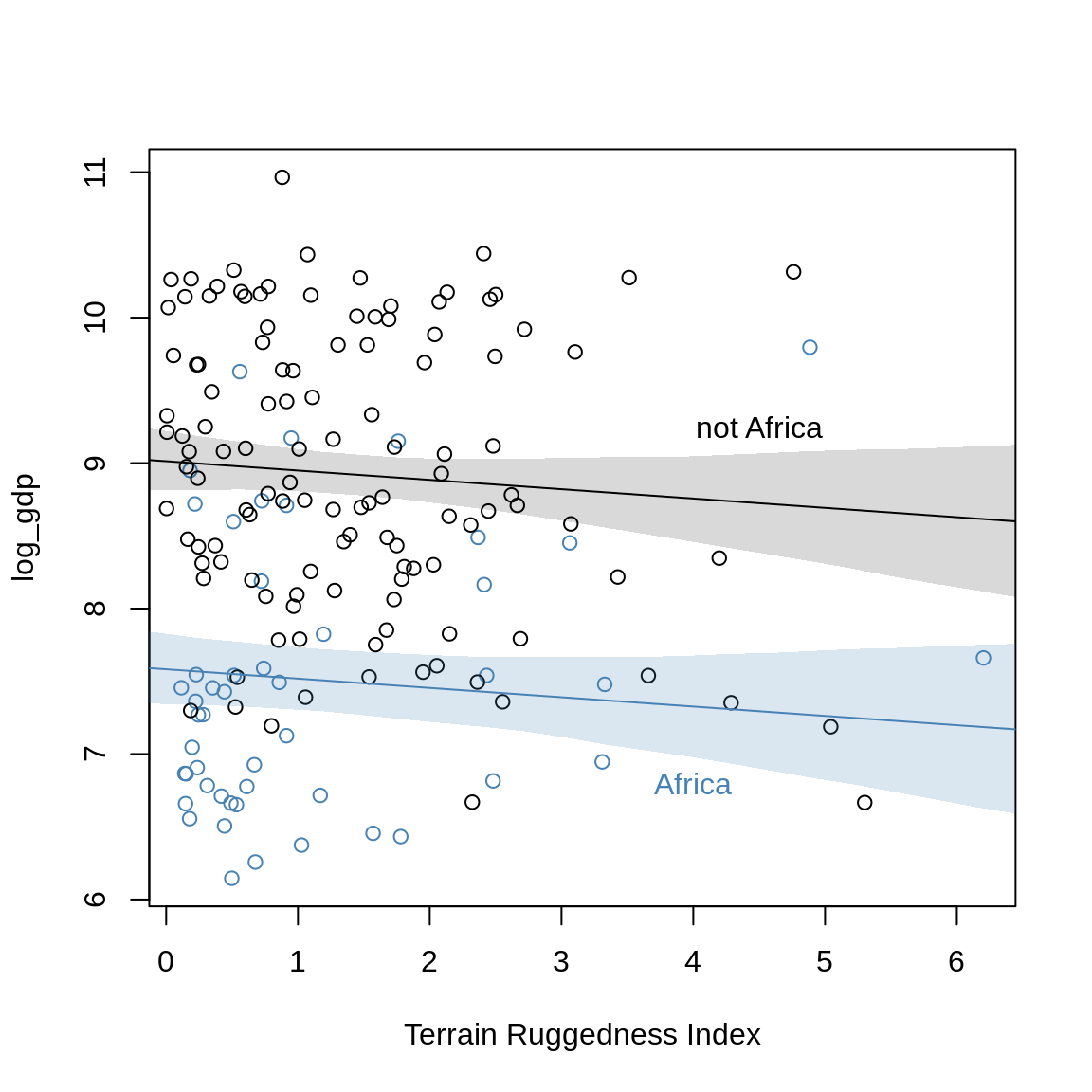
plot( precis(m7.5) )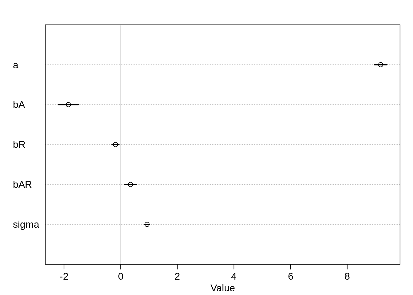
Gamma wasn’t estimated, we have to compute it ourselves.
post <- extract.samples( m7.5 )
gamma.Africa <- post$bR + post$bAR*1
gamma.notAfrica <- post$bR + post$bAR*0

mean( gamma.Africa )
## [1] 0.1646931mean( gamma.notAfrica )## [1] -0.1843582How do the distributions compare?
dens( gamma.Africa, xlim=c(-0.5, 0.6), ylim=c(0, 5.5),
      xlab="gamma", col="steelblue" )
dens( gamma.notAfrica, add=TRUE )
legend("topright", col=c("black", "steelblue"), bty="n",
       legend=c("not Africa", "Africa"), lty=c(1,1))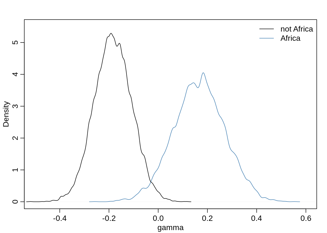
diff <- gamma.Africa - gamma.notAfrica
sum( diff < 0 ) / length( diff )
## [1] 0.0033So there is a very low probability that the African slope is less than the Non-African slope.
7.2 Symmetry of the linear interaction
The above interaction can be interpreted in two ways: (1) How much does the influence of ruggedness (on GDP) depend upon whether the nation is in Africa? (2) How much does the influence of being in Africa (on GDP) depend upon ruggedness?
Above, we plotted the first interpretation, which probably seems more natural for most. Let’s plot the other one:
q.rugged <- range(dd$rugged)

mu.ruggedlo <- link( m7.5,
                     data=data.frame(rugged=q.rugged[1], cont_africa=0:1) )
mu.ruggedlo.mean <- apply(mu.ruggedlo, 2, mean)
## Error in apply(mu.ruggedlo, 2, mean): dim(X) must have a positive lengthmu.ruggedlo.PI <- apply(mu.ruggedlo, 2, PI)## Error in apply(mu.ruggedlo, 2, PI): dim(X) must have a positive lengthmu.ruggedhi <- link( m7.5,
data=data.frame(rugged=q.rugged[2], cont_africa=0:1 ) )
mu.ruggedhi.mean <- apply(mu.ruggedhi, 2, mean )## Error in apply(mu.ruggedhi, 2, mean): dim(X) must have a positive lengthmu.ruggedhi.PI <- apply(mu.ruggedhi, 2, PI)## Error in apply(mu.ruggedhi, 2, PI): dim(X) must have a positive length# plot everything
med.r <- median(dd$rugged)
ox <- ifelse(dd$rugged > med.r, 0.05, -0.05 )
plot( dd$cont_africa + ox, dd$log_gdp,
col=ifelse(dd$rugged > med.r, "steelblue", "black"),
xlim = c(-0.25, 1.25), xaxt="n",
ylab ="log GDP year 2000",
xlab = "Continent")
axis(1, at=c(0, 1), labels=c("other", "Africa"))
lines(0:1, mu.ruggedlo.mean, lty=2)## Error in xy.coords(x, y): object 'mu.ruggedlo.mean' not foundtext(0.35, 9.4, "Low ruggedness", col="black")
shade(mu.ruggedlo.PI, 0:1 )## Error in shade(mu.ruggedlo.PI, 0:1): object 'mu.ruggedlo.PI' not foundlines(0:1, mu.ruggedhi.mean, col="steelblue")## Error in xy.coords(x, y): object 'mu.ruggedhi.mean' not foundshade(mu.ruggedhi.PI, 0:1, col=col.alpha("steelblue"))## Error in shade(mu.ruggedhi.PI, 0:1, col = col.alpha("steelblue")): object 'mu.ruggedhi.PI' not foundtext(0.35, 7.3, "High ruggedness", col="steelblue")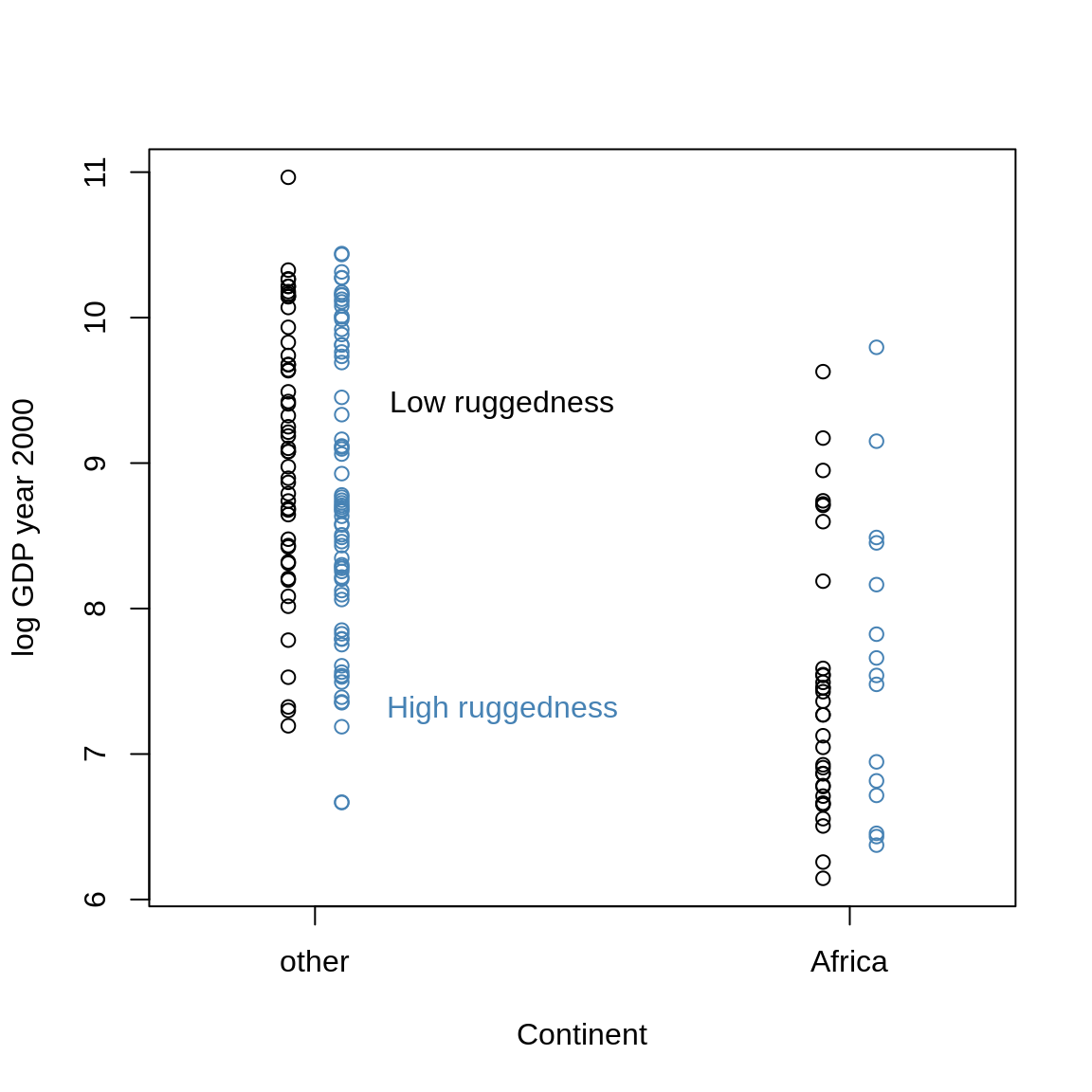
Blue points are nations with above-median ruggedness. Black points are below the median. The dashed black line is the relationship between continent and log-GDP for an imaginary nation with minimum observed ruggedness (0.003). The blue line is an imaginary nation with maximum observed ruggedness (6.2).
That is, if we have a nation with low ruggedness and we “move” it to Africa, it’s GDP goes down, whereas a nation with high ruggedness would see its GDP increase.
7.3 Continuous interactions
data(tulips)
d <- tulips
str(d)
## 'data.frame': 27 obs. of 4 variables:
## $ bed : Factor w/ 3 levels "a","b","c": 1 1 1 1 1 1 1 1 1 2 ...
## $ water : int 1 1 1 2 2 2 3 3 3 1 ...
## $ shade : int 1 2 3 1 2 3 1 2 3 1 ...
## $ blooms: num 0 0 111 183.5 59.2 ...Both water and light help plants grow and produce blooms, so we can model this as an interaction. The difficulty for continuous interactions is how to interpret them.
Let’s first implement two models, one with and one without interaction. This time, we use very flat priors.
m7.6 <- map(
  alist(
    blooms ~ dnorm(mu, sigma),
    mu <- a + bW*water + bS*shade,
    a ~ dnorm( 0, 100),
    bW ~ dnorm( 0, 100),
    bS ~ dnorm( 0, 100),
    sigma ~ dunif( 0, 100)
  ), data=d
)
## Caution, model may not have converged.## Code 1: Maximum iterations reached.m7.7 <- map(
alist(
blooms ~ dnorm( mu, sigma),
mu <- a + bW*water + bS*shade + bWS*water*shade,
a ~ dnorm(0, 100),
bW ~ dnorm( 0, 100),
bS ~ dnorm( 0, 100),
bWS ~ dnorm( 0, 100),
sigma ~ dunif( 0, 100)
), data=d
)## Error in map(alist(blooms ~ dnorm(mu, sigma), mu <- a + bW * water + bS * : non-finite finite-difference value [5]
## Start values for parameters may be too far from MAP.
## Try better priors or use explicit start values.
## If you sampled random start values, just trying again may work.
## Start values used in this attempt:
## a = 62.5704792195615
## bW = 0.71488832064561
## bS = 12.1726842940726
## bWS = -36.680326642862
## sigma = 97.0881580375135Fitting this code very likely produces errors: The flat priors make it hard for the optimizer to find good start values that converge. We can fix this problem different ways:
- use another optimizer
- search longer, that is raise the maximum iterations
- rescale the data to make it easier to find the right values
We first try the first two options:
m7.6 <- map(
  alist(
    blooms ~ dnorm(mu, sigma),
    mu <- a + bW*water + bS*shade,
    a ~ dnorm( 0, 100),
    bW ~ dnorm( 0, 100),
    bS ~ dnorm( 0, 100),
    sigma ~ dunif( 0, 100)
  ),
  data=d,
  method="Nelder-Mead",
  control=list(maxit=1e4)
)
## Error in map(alist(blooms ~ dnorm(mu, sigma), mu <- a + bW * water + bS * : non-finite finite-difference value [4]
## Start values for parameters may be too far from MAP.
## Try better priors or use explicit start values.
## If you sampled random start values, just trying again may work.
## Start values used in this attempt:
## a = -38.8981859721942
## bW = -105.492743759584
## bS = -73.4617528737223
## sigma = 25.7715692277998m7.7 <- map(
alist(
blooms ~ dnorm( mu, sigma),
mu <- a + bW*water + bS*shade + bWS*water*shade,
a ~ dnorm(0, 100),
bW ~ dnorm( 0, 100),
bS ~ dnorm( 0, 100),
bWS ~ dnorm( 0, 100),
sigma ~ dunif( 0, 100)
),
data=d,
method="Nelder-Mead",
control=list(maxit=1e4)
)No more warnings this time.
coeftab(m7.6, m7.7)## Caution, model may not have converged.## Code 1: Maximum iterations reached.## Caution, model may not have converged.## Code 1: Maximum iterations reached.## m7.6 m7.7
## a 55.10 -203.32
## bW 75.96 201.88
## bS -39.32 90.47
## sigma 57.28 55.04
## bWS NA -63.2
## nobs 27 27plot( coeftab( m7.6, m7.7 ) )## Caution, model may not have converged.## Code 1: Maximum iterations reached.## Caution, model may not have converged.## Code 1: Maximum iterations reached.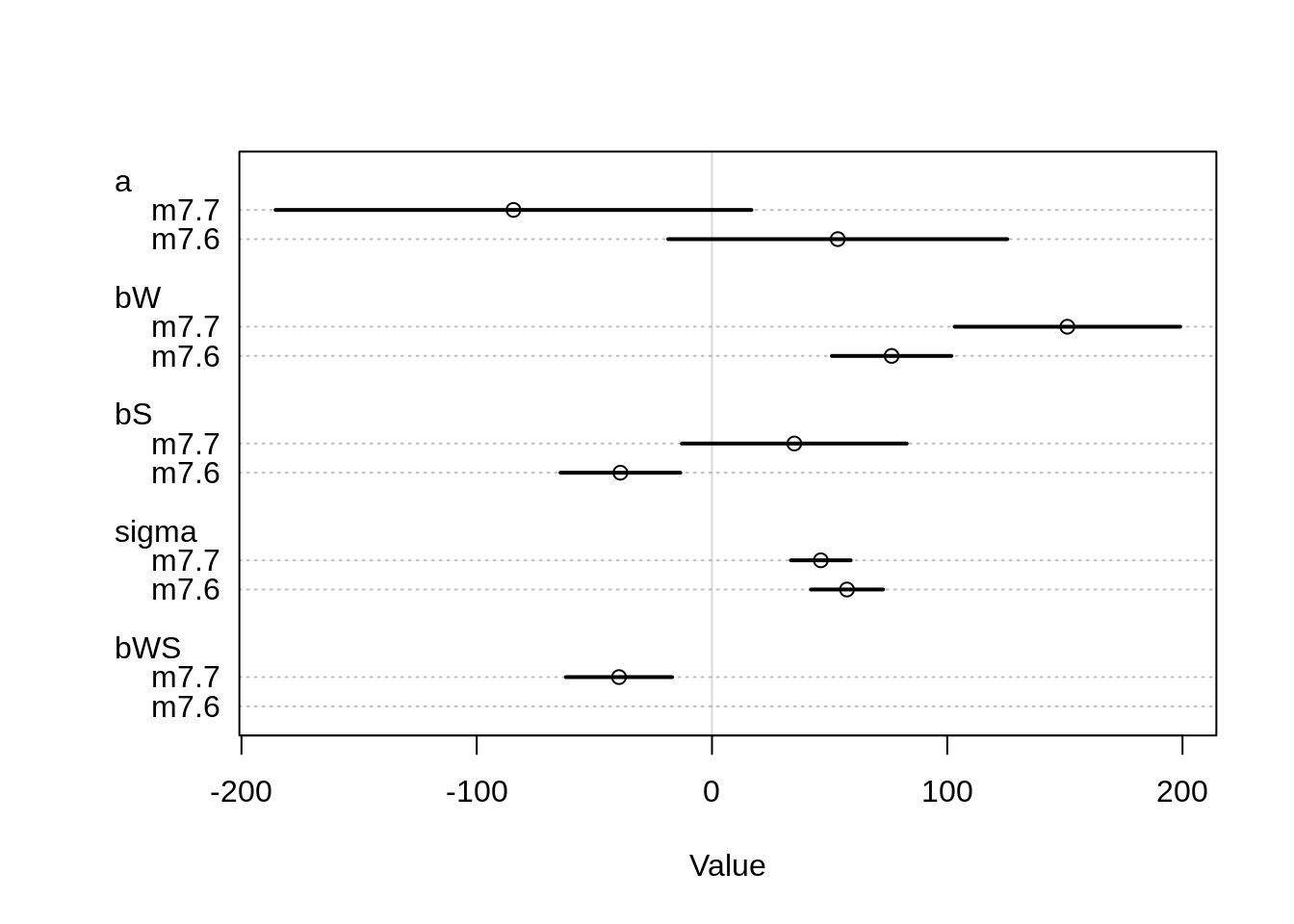
The estimates are all over the place… The intercept changes from positive to negative in the second model. In the first model, both the water and shade coefficient are as expected: more water, more blooms and more shade less blooms. For shade, the influence actually becomes positive in the second model. The estimates are not that easy to understand and shouldn’t be taken at face value.
compare( m7.6, m7.7 )## WAIC SE dWAIC dSE pWAIC weight
## m7.7 300.2630 9.482958 0.000000 NA 7.155731 0.96084845
## m7.6 306.6638 9.347944 6.400753 9.429719 5.696026 0.03915155Pretty much all weight is on the second model with interaction term, so it seems to be a better model than without interaction term.
Center and re-estimate
Now, let’s center the variables instead.
d$shade.c <- d$shade - mean(d$shade)
d$water.c <- d$water - mean(d$water)
Run the models again:
m7.8 <- map(
  alist(
    blooms ~ dnorm( mu, sigma),
    mu <- a + bW*water.c + bS*shade.c ,
    a ~ dnorm( 0, 100),
    bW ~ dnorm( 0, 100),
    bS ~ dnorm( 0, 100),
    sigma ~ dunif( 0, 100)
  ),
  data=d,
  start=list(a=mean(d$blooms), bW=0, bS=0, sigma=sd(d$blooms))
)
m7.9 <- map(
  alist(
    blooms ~ dnorm( mu, sigma),
    mu <- a + bW*water.c + bS*shade.c + bWS*water.c*shade.c,
    a ~ dnorm(0, 100),
    bW ~ dnorm( 0, 100),
    bS ~ dnorm( 0, 100),
    bWS ~ dnorm( 0, 100),
    sigma ~ dunif( 0, 100)
  ),
  data=d,
  start=list(a=mean(d$blooms), bW=0, bS=0, bWS=0,
             sigma=sd(d$blooms))
)
coeftab( m7.8, m7.9)
## m7.8 m7.9
## a 127.44 128.05
## bW 74.43 74.95
## bS -40.85 -41.13
## sigma 57.37 45.23
## bWS NA -51.83
## nobs 27 27plot( coeftab( m7.8, m7.9 ))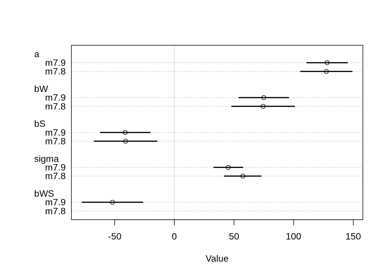
The estimates for both models look more reasonable: The intercept for both models is the same, it now corresponds to the average bloom. The influence of shade is also negative in both models now.
mean(d$bloom)## [1] 128.9937Just the estimates of the interaction model:
precis( m7.9 )## mean sd 5.5% 94.5%
## a 128.05308 8.675182 114.18846 141.91769
## bW 74.94620 10.602917 58.00069 91.89171
## bS -41.13326 10.601175 -58.07599 -24.19054
## bWS -51.83366 12.949359 -72.52923 -31.13808
## sigma 45.22859 6.154896 35.39188 55.06530Plot continuous interactions
Let’s plot the predictions. We make a plot showing the predictions for different values of water to get a feeling of the interaction effect.
par(mfrow=c(2,3))

shade.seq <- -1:1
# plot for model m7.8
for ( w in -1:1 ){
  dt <- d[d$water.c==w, ]
  plot(blooms ~ shade.c, data=dt, col="steelblue",
       main=paste("water.c = ", w), xaxp=c(-1,1,2),
       ylim=c(0, 362), xlab="shade (centered)")
  mu <- link( m7.8, data=data.frame(water.c=w, shade.c=shade.seq ) )
  mu.mean <- apply(mu, 2, mean)
  mu.PI <- apply( mu, 2, PI)
  lines( shade.seq, mu.mean )
  lines( shade.seq, mu.PI[1,], lty=2 )
  lines( shade.seq, mu.PI[2,], lty=2)
}

# plot for model m7.9
for ( w in -1:1 ){
  dt <- d[d$water.c==w, ]
  plot(blooms ~ shade.c, data=dt, col="steelblue",
       main=paste("water.c = ", w), xaxp=c(-1,1,2),
       ylim=c(0, 362), xlab="shade (centered)")
  mu <- link( m7.9, data=data.frame(water.c=w, shade.c=shade.seq ) )
  mu.mean <- apply(mu, 2, mean)
  mu.PI <- apply( mu, 2, PI)
  lines( shade.seq, mu.mean )
  lines( shade.seq, mu.PI[1,], lty=2 )
  lines( shade.seq, mu.PI[2,], lty=2)
}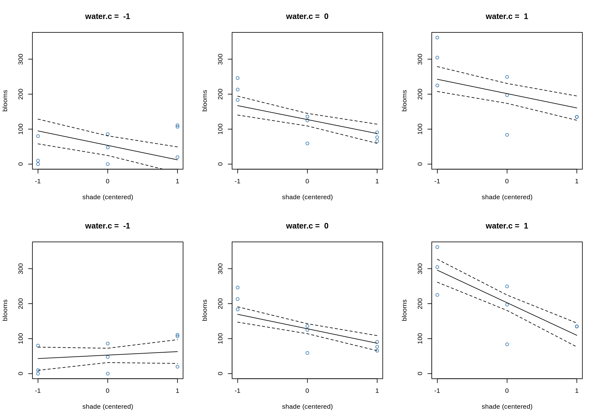
In the top row, the model without the interaction, the slope for shade does not change, only the intercept. In the bottom row, the influence of shade changes, depending on how much water there is. If there is little water, the plant can’t grow well, so no shade or a lot of shade doesn’t change the bloom much. Whereas, if we have a more water, shade has a big difference, noticeably in the steep slope. In all plots, the blue points are the data points that had the corresponding water value.
We can also visualize this the other way round:
par(mfrow=c(2,3))

water.seq <- -1:1
# plot for model m7.8
for ( s in -1:1 ){
  dt <- d[d$shade.c==s, ]
  plot(blooms ~ water.c, data=dt, col="steelblue",
       main=paste("shade.c = ", s), xaxp=c(-1,1,2),
       ylim=c(0, 362), xlab="water (centered)")
  mu <- link( m7.8, data=data.frame(water.c=water.seq, shade.c=s ) )
  mu.mean <- apply(mu, 2, mean)
  mu.PI <- apply( mu, 2, PI)
  lines( shade.seq, mu.mean )
  lines( shade.seq, mu.PI[1,], lty=2 )
  lines( shade.seq, mu.PI[2,], lty=2)
}

# plot for model m7.9
for ( s in -1:1 ){
  dt <- d[d$shade.c==s, ]
  plot(blooms ~ water.c, data=dt, col="steelblue",
       main=paste("shade.c = ", s), xaxp=c(-1,1,2),
       ylim=c(0, 362), xlab="water (centered)")
  mu <- link( m7.9, data=data.frame(water.c=water.seq, shade.c=s ) )
  mu.mean <- apply(mu, 2, mean)
  mu.PI <- apply( mu, 2, PI)
  lines( shade.seq, mu.mean )
  lines( shade.seq, mu.PI[1,], lty=2 )
  lines( shade.seq, mu.PI[2,], lty=2)
}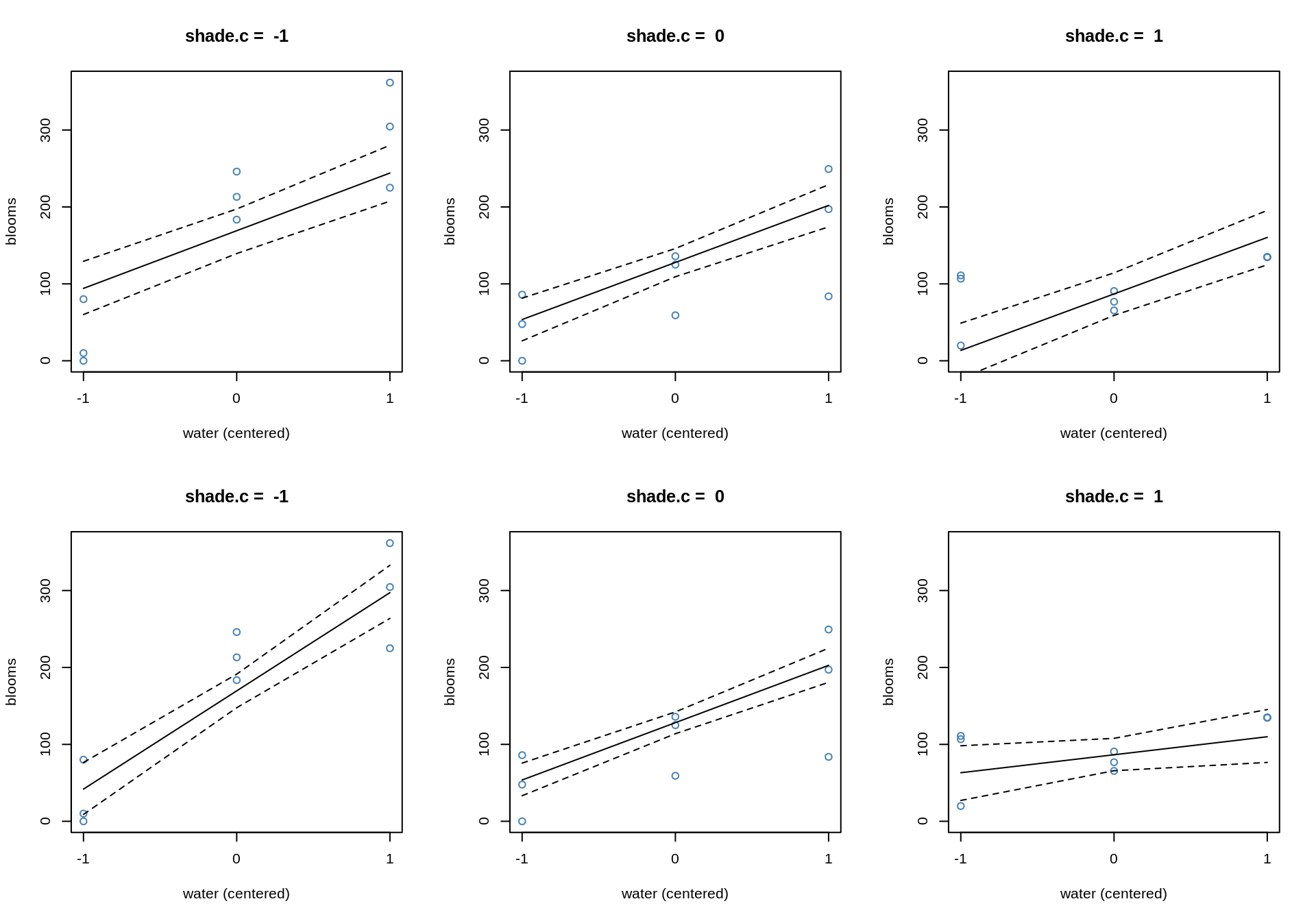
7.4 Interactions in design formulas
m7.x <- lm( y ~ x + z + x*z, data=d)Same model:
m7.x <- lm( y ~ x*z, data=d)Fit a model with interaction term but without direct effect:
m7.x <- lm( y ~ x + x*z - z, data=d)Run a model with interaction term and all lower-order interactions:
m7.x <- lm( y ~ x*z*w, data=d)corresponds to \[\begin{align*} y_i &\sim \text{Normal}(\mu_i, \sigma) \\ \mu_i &= \alpha + \beta_x x_i + \beta_z z_i + \beta_w w_i + \beta_{xz} x_i z_i + \beta_{xw} x_i w_i + \beta_{zw} z_i w_w + \beta_{xzw} x_i z_i w_i \end{align*}\]
You can also get direct access to the function used by lm to expand these formulas:
x <- z <- w <- 1
colnames( model.matrix(~ x*z*w ))
## [1] "(Intercept)" "x" "z" "w" "x:z"
## [6] "x:w" "z:w" "x:z:w"where : stands for multiplication.