The Problem with Dummies

In the simplest case we only have two categories, e.g. male and female. We are going to use the Kalahari data again to illustrate how to add binary categorical variables.

library(rethinking)
data("Howell1")
d <- Howell1
str(d)

'data.frame':   544 obs. of  4 variables:
 $ height: num  152 140 137 157 145 ...
 $ weight: num  47.8 36.5 31.9 53 41.3 ...
 $ age   : num  63 63 65 41 51 35 32 27 19 54 ...
 $ male  : int  1 0 0 1 0 1 0 1 0 1 ...

There is the variable male that consists of 0’s and 1’s. It is 1 if the individual is male and 0 if female. This is called an Indicator Variable or in an ML context also known as Dummy Variable. One way to include the male variable in our model is to use the indicator variable directly:

\[\begin{align*} h_i &\sim \text{Normal}(\mu_i, \sigma) \\ \mu_i &= \alpha + \beta_m m_i \\ \alpha &\sim \text{Normal}(178, 20) \\ \beta_m &\sim \text{Normal}(0, 10) \\ \sigma &\sim \text{Uniform}(0, 50) \end{align*}\]

Now what happens in this model? If \(m_i = 0\), that is, an individual is female, then the \(\beta_m m_i\) term is 0 and the predicted mean (for women) is \(\alpha\). If however \(m_i = 1\) then the predicted mean (for men) is \(\alpha + \beta_m\). This means \(\alpha\) does not represent the average height of the total population anymore but the average height for one of our categories, in this case the female category. \(\beta_m\) then gives us the difference between average female and average male height.

This can make it harder to assign sensible priors. We can’t just assign the same prior for each category since one category is encoded in \(\alpha\) and the other category is encoded as the difference in the slope \(\beta\).

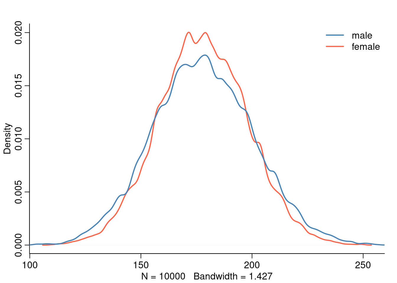
Another important point to take into account with this approach is that we assume more uncertainty for male height. The male height is constructed from two parameters and two priors and thus has more uncertainty than female height which only uses one parameter and one prior.

Let’s simulate this from the prior:

mu_female <- rnorm( 1e4, 178, 20 )
mu_male <- rnorm( 1e4, 178, 20 ) + rnorm( 1e4, 0, 10 )
precis( data.frame( mu_female, mu_male ))

	mean	sd	5.5%	94.5%	histogram
mu_female	178	20.0	146	210	▁▁▁▂▃▇▇▇▅▃▁▁▁▁
mu_male	178	22.7	142	215	▁▁▁▃▇▇▃▁▁

The standard deviation of mu_male is slightly higher than the one for mu_female.

The Index Variable Approach

Instead of using dummy variables, we can also use an index variable.

d$sex <- ifelse( d$male == 1, 2, 1)
str(d$sex)

 num [1:544] 2 1 1 2 1 2 1 2 1 2 ...

We assign each category an integer. In this example “1” means female and “2” means male. The ordering doesn’t matter, it could be either way, the integers are just labels (that are easier to read for the machine than strings). The mathematical model to incorporate this variable than looks like this: \[\begin{align*} h_i &\sim \text{Normal}(\mu_i, \sigma) \\ \mu_i &= \alpha_{sex[i]} \\ \alpha_j &\sim \text{Normal}(178, 20) \\ \beta_m &\sim \text{Normal}(0, 10) \\ \sigma &\sim \text{Uniform}(0, 50) \end{align*}\]

We now fit one \(\alpha\) parameter for each category so \(\alpha\) is actually a vector consisting of \(\alpha_1\) and \(\alpha_2\). Now we can assign the same prior to both categories.

Let’s fit this model:

m5.8 <- quap(
  alist(
    height ~ dnorm( mu, sigma ),
    mu <- a[sex],
    a[sex] ~ dnorm( 178, 20),
    sigma ~ dunif(0, 50)
  ), data = d
)
precis( m5.8, depth = 2)

	mean	sd	5.5%	94.5%
a[1]	134.9	1.607	132	137.5
a[2]	142.6	1.697	140	145.3
sigma	27.3	0.828	26	28.6

Now the interpretation of the parameters is also easier: a[1] is the average height for women and a[2] is the average height for men, no need to first compute the difference. If we are interested in the difference, we can directly calculate it like this from the posterior:

post <- extract.samples( m5.8 )
post$diff_fm <- post$a[,1] - post$a[,2]
precis( post, depth = 2)

	mean	sd	5.5%	94.5%	histogram
sigma	27.32	0.826	26.0	28.64	▁▁▁▁▃▅▇▇▃▂▁▁▁
a[1]	134.92	1.614	132.4	137.54	▁▁▁▁▂▅▇▇▅▂▁▁▁
a[2]	142.59	1.716	139.8	145.35	▁▁▁▂▃▇▇▇▃▂▁▁▁▁
diff_fm	-7.67	2.375	-11.5	-3.88	▁▁▁▃▇▇▃▁▁▁

This kind of calculation, computing the difference, is also called a contrast.

More Categories

Very often, we have more than two categories. If we wanted to use the indicator approach, we have to add new variables for each category but one. So if there are \(k\) categories, we’d need \(k-1\) dummy variables. This can very quickly become unfeasible and it also is difficult to assign reasonable priors to each. The index approach scales better in this case.

Let’s show this with an example using the milk data.

data(milk)
d <- milk
levels(d$clade)

[1] "Ape"              "New World Monkey" "Old World Monkey" "Strepsirrhine"   

The variable clade encodes the taxonomy membership of each species. We can compute an index variable as follow:

d$clade_id <- as.integer(d$clade)

We will fit this mathematical model: \[\begin{align*} K_i &\sim \text{Normal}(\mu_i, \sigma)\\ \mu_i &= \alpha_{CLADE[i]} & \text{for } j = 1..4\\ \alpha_j &\sim \text{Normal}(0, 0.5) \\ \sigma &\sim \text{Exponential}(1) \end{align*}\] And in R:

d$K <- standardize( d$kcal.per.g )
m5.9 <- quap(
  alist(
    K ~ dnorm( mu, sigma) ,
    mu <- a[clade_id],
    a[clade_id] ~ dnorm(0, 0.5),
    sigma ~ dexp(1)
  ), data=d
)
labels <- paste( "a[", 1:4, "]: ", levels(d$clade), sep="")
plot(precis( m5.9, depth=2, pars="a"), labels = labels,
     xlab = "expected kcal (std)")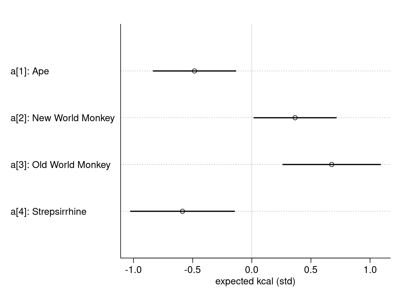

Even More Categories

We can also add more than one categorical variable. Imagine, these primates would be sorted into the Harry Potter houses: [1] Gryffindor, [2] Hufflepuff, [3] Ravenclaw, [4] Slytherin. We could add this variable as follow:

set.seed(63)
d$house <- sample( rep(1:4, each = 8), size=nrow(d))
m5.10 <- quap(
  alist(
    K ~ dnorm( mu, sigma),
    mu <- a[clade_id] + h[house],
    a[clade_id]  ~ dnorm(0, 0.5),
    h[house] ~ dnorm(0, 0.5),
    sigma ~ dexp(1)
  ), data=d
)

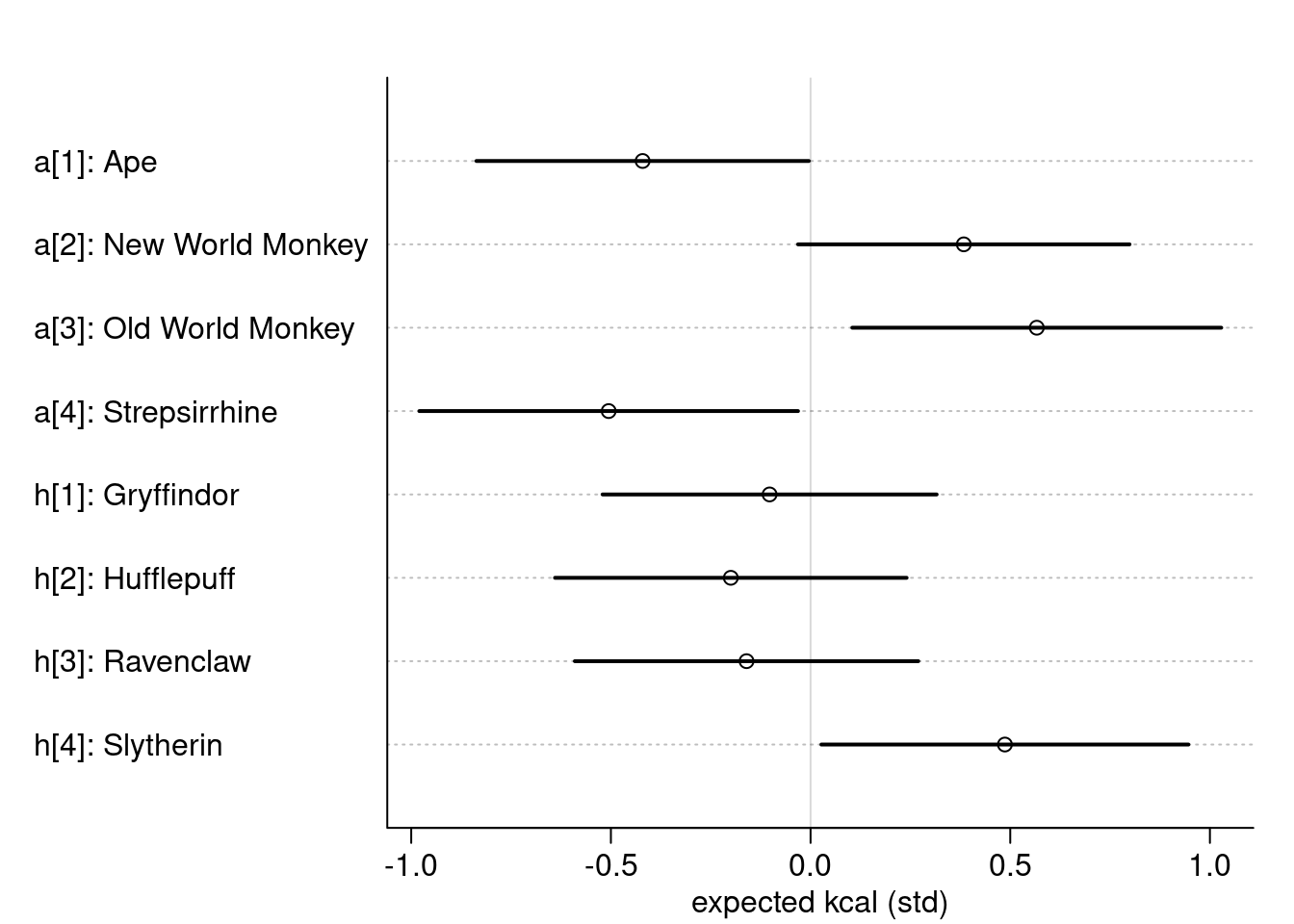
Using this random seed, only Slytherin has an effect on the expected kcal.

Notes of Caution

There are a few things to be aware of when working with categorical variables:

• Don’t accidentally encode your categorical variables in the model as continuous. If we’d for example use the index variable for the clade variable in the model, this would apply that New World Monkeys are somehow twice as “clade” as Apes. This is obviously meaningless.
• If two categories are both different from 0 this still does not mean that there difference is different from 0. Same when having two categories where only one is far away from zero. The difference might still not be “significant”. We always must compute the difference explicitly using the posterior.
• Categories are itself a model decision. Nothing in the world is really categorical and pretty much all categorical variables are man-made. When working with survey data for example, using only male and female as categories might not be enough and e.g. non-binary should be added. Categorization can also have funny side-effects such as when deciding for kids in which group they compete in sports. If the birth year is used, kids born early in the year have an advantage over kids born later in the year and thus sport stars are more often born in January.
  Sometimes, it can make sense to merge categories. This should always be guided by scientific theory and not by if a category is significant or not.

Full code.