Over-dispersed outcomes

For the beta-binomial model, we’ll make use of the beta distribution. The beta distribution is a probability distribution over probabilities (over the interval \([0, 1]\)).

library(rethinking)
pbar <- 0.5
theta <- 5
curve( dbeta2( x, pbar, theta), from=0, to=1, xlab="probability", ylab="Density")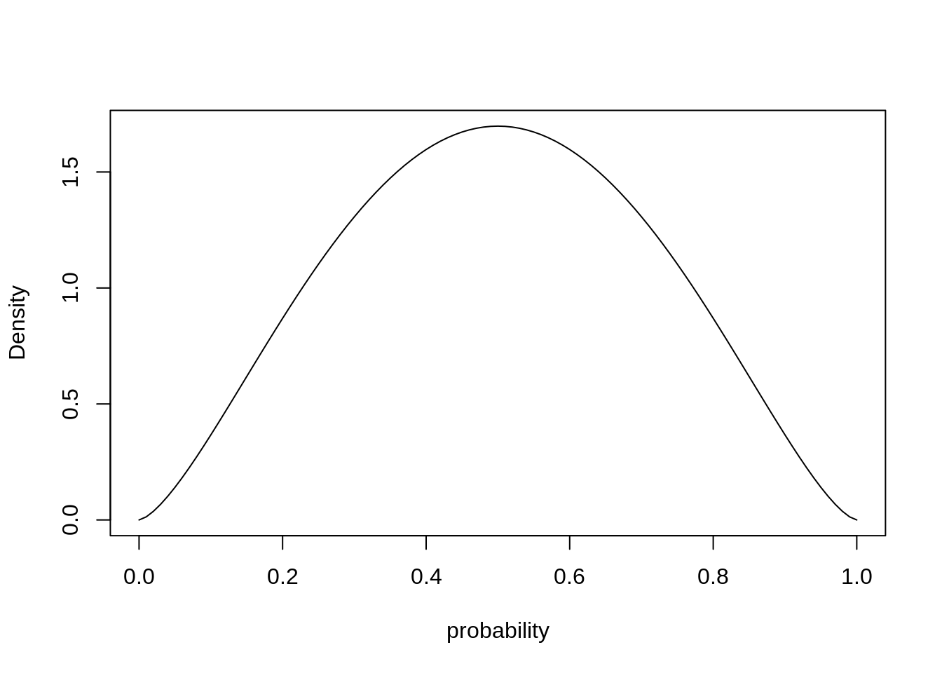

There are different ways to parametrize the beta distribution:

dbeta2 <- function( x , prob , theta , log=FALSE ) {
    a <- prob * theta
    b <- (1-prob) * theta
    dbeta( x , shape1=a , shape2=b , log=log )
}

We use the beta-binomial for the UCBadmit data, which is over-dispersed if we ignore department (since the admission rate varied quite a lot for different departments). Our model looks as follows: \[\begin{align*} A_i &\sim \text{BetaBinomial}(N_i, \bar{p}_i, \theta) \\ \text{logit}(\bar{p}_i) &= \alpha_{\text{GID}[i]}) \\ \alpha_j &\sim \text{Normal}(0, 1.5) \\ \theta &\sim \text{Exponential}(1) \end{align*}\] where \(A\) is admit, \(N\) is the number of applications applications, and GID\([i]\) is gender id, 1 for male and 2 for female.

data("UCBadmit")
d <- UCBadmit
d$gid <- ifelse(d$applicant.gender == "male", 1L, 2L)
dat <- list(A = d$admit, N = d$applications, gid=d$gid)

m12.1 <- ulam(
  alist(
    A ~ dbetabinom( N, pbar, theta),
    logit(pbar) <- a[gid],
    a[gid] ~ dnorm(0, 1.5),
    theta ~ dexp(1)
  ), data=dat, chains=4
)

post <- extract.samples(m12.1 )
post$da <- post$a[,1] - post$a[,2]
precis( post, depth=2)

            mean        sd       5.5%     94.5%  histogram
a[1]  -0.4170432 0.4327273 -1.1055429 0.2583752    ▁▂▇▇▂▁▁
a[2]  -0.3063994 0.4285321 -0.9805098 0.4067581    ▁▁▅▇▃▁▁
theta  2.6763961 0.9493179  1.3789576 4.2942542  ▁▃▇▃▁▁▁▁▁
da    -0.1106438 0.5862838 -1.0271344 0.8384815 ▁▁▁▃▇▇▂▁▁▁

a[1] is the log-odds of admission for male applicants which is lower than a[2], the log-odds for female applicants. This might suggest there is a diffenrece in admission rates by gender, but the posterior difference da is highly uncertain with probability mass both above and below zero.

We can visualize the posterior Beta-distribution:

gid <- 2
# draw posterior mean beta distribution
curve( dbeta2(x, mean( logistic(post$a[, gid])), mean(post$theta)), from=0, to=1,
       ylab="Density", xlab="probability admit", ylim=c(0,3), lwd=2)

# draw 50 beta distributions sampled from posterior
for ( i in 1:50 ) {
  p <- logistic( post$a[i, gid ] )
  theta <- post$theta[i]
  curve( dbeta2(x, p, theta), add=T,col=col.alpha("black", 0.2))
}
mtext("distribution of female admission rates")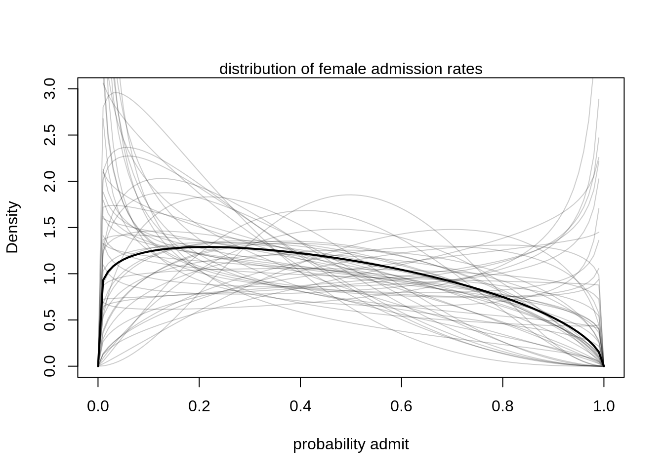

There is a tendency for admission rates below 40% but the most plausible (the mean Beta-distribution) also allows for very high admission rates above 80%. This way, the model incorporated the high variation among departments.

postcheck(m12.1)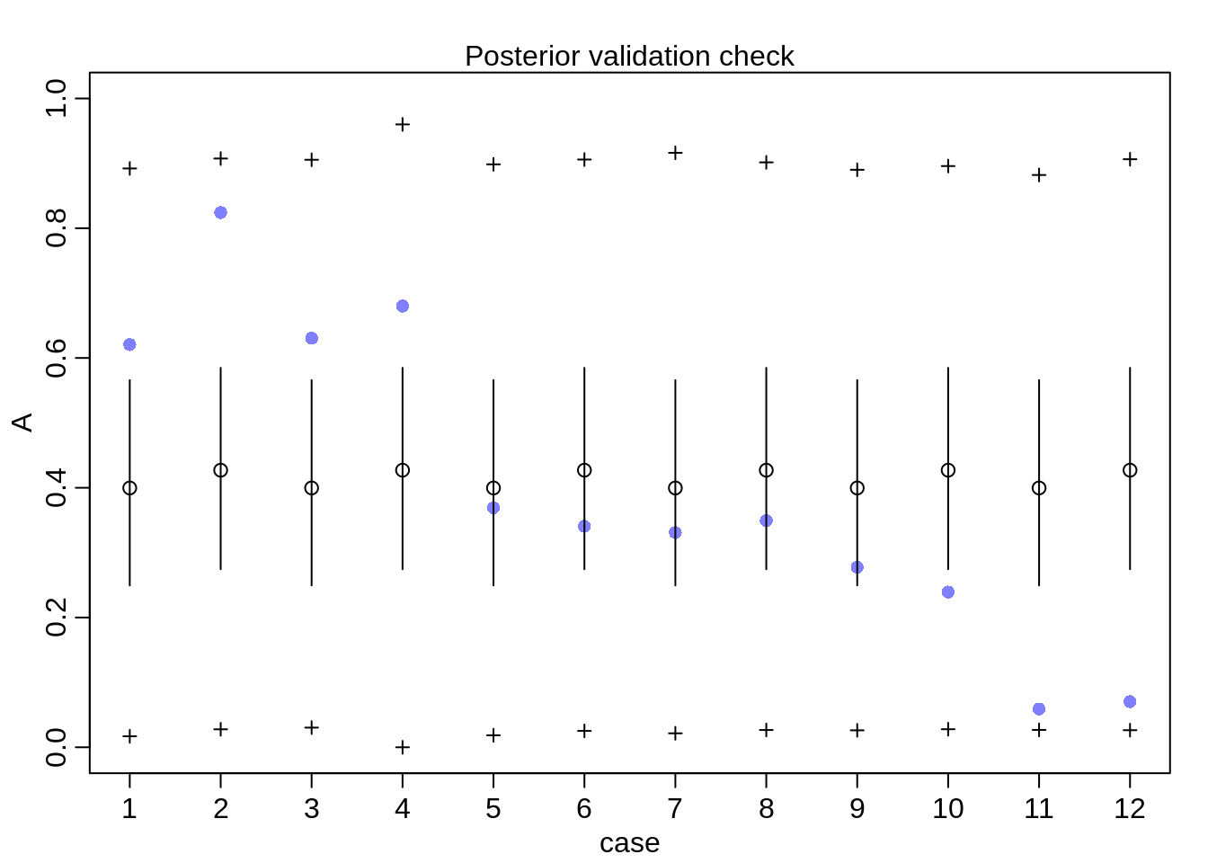

The prediction intervals are very wide, the model incorporated such a wide variance since even though it doesn’t see the different departments, it does see heterogeneity across rows.

Negative-Binomial

Similar as with the Beta-Binomial, we can fit a Poisson model, where each observation has its own rate. The rate comes from a common gamma distribution.

phi <- 2
lambda <- 1
curve( dgamma( x, shape=phi, rate=lambda), from=0, to=20, xlab="rate", ylab="probability density")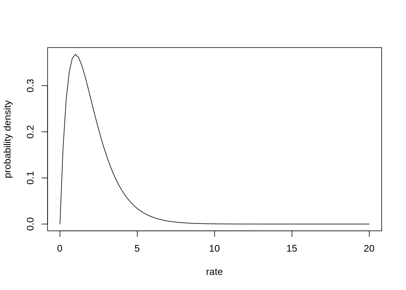

We check again the Kline data of the tool counts for different islands, this time using the negative-binomial model.

data(Kline)
d <- Kline
d$P <- standardize( log( d$population ) )
d$contact_id <- ifelse( d$contact == "high", 2L, 1L)

dat2 <- list(
  TT = d$total_tools,
  P = d$population,
  cid = d$contact_id
)

m12.3 <- ulam(
  alist(
    TT ~ dgampois( lambda, phi ),
    lambda <- exp( a[cid])*P^b[cid] / g,
    a[cid] ~ dnorm(1, 1),
    b[cid] ~ dexp(1),
    g ~ dexp(1),
    phi ~ dexp(1)
  ), data=dat2, chains=4, log_lik = TRUE
)

For comparison, we also fit our model from before, using a pure Poisson model.

m11.11 <- ulam(
  alist(
    TT ~ dpois(lambda),
    lambda <- exp( a[cid] )*P^b[cid] / g,
    a[cid] ~ dnorm(1,1),
    b[cid] ~ dexp(1),
    g ~ dexp(1)
  ), data=dat2, chains=4, log_lik = T
)

k <- PSIS( m11.11 , pointwise=TRUE )$k
par(bty="l", mfrow=c(1,2))
plot( d$population, d$total_tools, xlab="population", ylab="total tools",
      col=rangi2, pch=ifelse(dat2$cid == 1, 1, 16), lwd=2,
      ylim=c(0,74), cex=1+normalize(k) )

ns <- 100
P_seq <- seq(from=0, to=12.55, length.out = ns)
pop_seq <- exp( P_seq )

lambda <- link(m12.3, data=data.frame(P = pop_seq, cid=1))
lmu <- apply(lambda, 2, mean)
lci <- apply(lambda, 2, PI )
lci2 <- ifelse(lci >= 74, 74, lci)
lines( pop_seq, ifelse(lmu>=74, NA, lmu), lty=2, lwd=1.5)
shade(lci2, pop_seq, xpd=TRUE)

lambda <- link(m12.3, data=data.frame(P = pop_seq, cid=2))
lmu <- apply(lambda, 2, mean)
lci <- apply(lambda, 2, PI )
lci2 <- ifelse(lci >= 74, 74, lci)
lines( pop_seq, ifelse(lmu>=74, NA, lmu), lty=1, lwd=1.5)
shade(lci2, pop_seq, xpd=TRUE)
text(c(9e4, 1e5), c(68, 50), labels=c("high contact", "low contact"))
mtext("gamma-Poisson model")


plot( d$population, d$total_tools, xlab="population", ylab="total tools",
      col=rangi2, pch=ifelse(dat2$cid == 1, 1, 16), lwd=2,
      ylim=c(0,74), cex=1+normalize(k) )

lambda <- link(m11.11, data=data.frame(P = pop_seq, cid=1))
lmu <- apply(lambda, 2, mean)
lci <- apply(lambda, 2, PI )
lci2 <- ifelse(lci >= 74, 74, lci)
lines( pop_seq, ifelse(lmu>=74, NA, lmu), lty=2, lwd=1.5)
shade(lci2, pop_seq, xpd=TRUE)

lambda <- link(m11.11, data=data.frame(P = pop_seq, cid=2))
lmu <- apply(lambda, 2, mean)
lci <- apply(lambda, 2, PI )
lci2 <- ifelse(lci >= 74, 74, lci)
lines( pop_seq, ifelse(lmu>=74, NA, lmu), lty=1, lwd=1.5)
shade(lci2, pop_seq, xpd=TRUE)
mtext("pure Poisson model")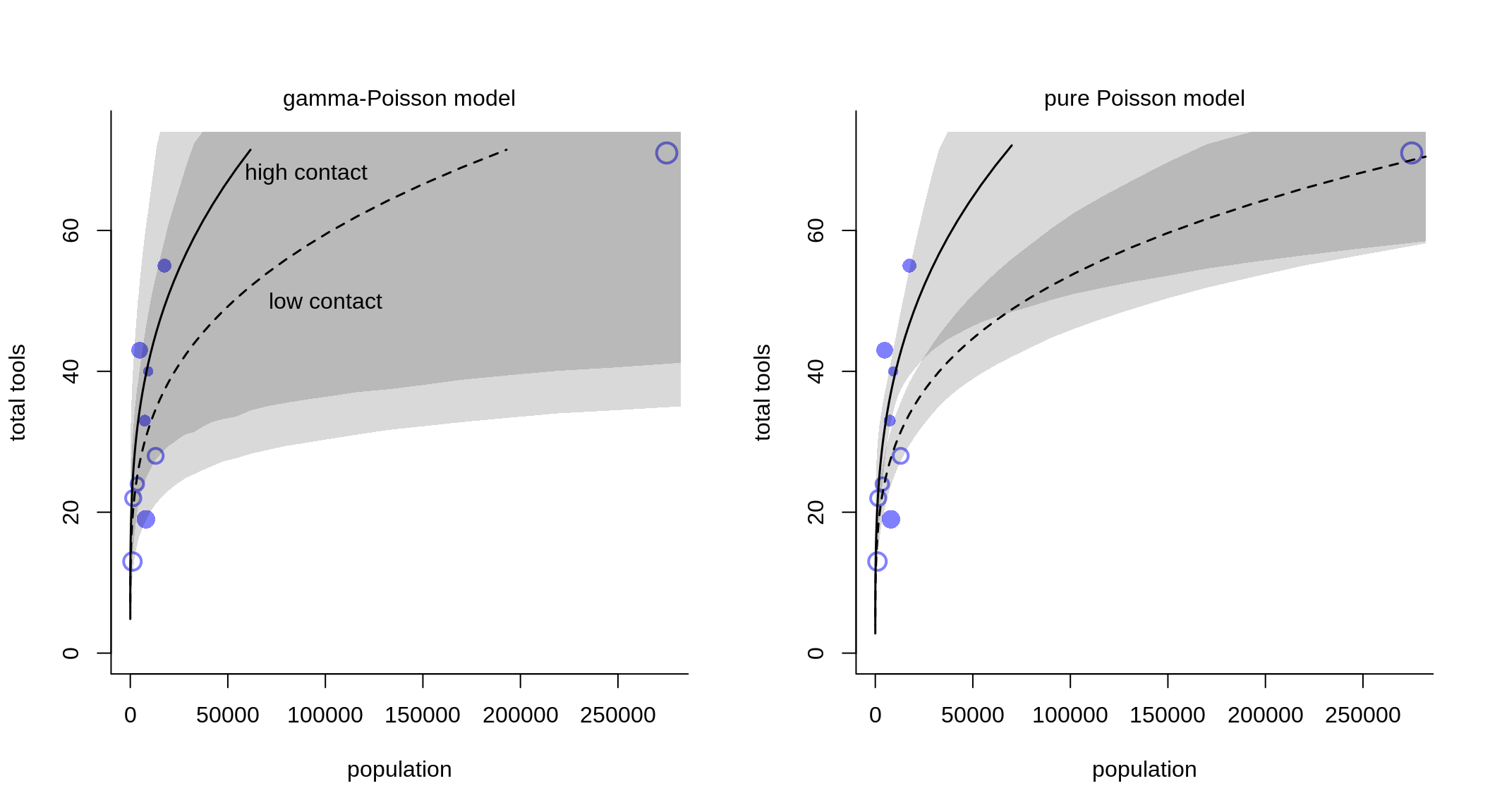

Again, we can see that the mixture model incorporates much more uncertainty compared to the pure, non-mixed model.

Zero-inflated outcomes

Often, the things we measure are not from any pure process but rather mixtures of different processes. One such example is count data. Very often a count of zero can happen in more than one way: either the rate of processes is low or the process that generates events failed to start in the first place.

If we go back to our example of monks writing manuscripts. Many monks work on manuscripts and on some days, they’ll finish a few. The rate is thus very low and there will be days where no manuscript is finished. However, imagine that on some days, the monks take a break and instead of writing, they open the wine cellar. On these days, no manuscript will be produced. So we have two ways how we end up with a count of no manuscripts.

Let’s simulate this process. We assume that the probability on any day that the monks are drinking instead of working is 20%. The rate at which they produce manuscripts is one manuscript per day.

prob_drink <- 0.2
rate_work <- 1

We simulate counts for one whole year. First, for each day we simulate using a binomial process, if the monks were drinking or working.

N <- 365
set.seed(365)
drink <- rbinom( N, 1, prob_drink)

Next, for each day we simulate how many manuscripts the monks would have finished and multiply with 0 if on a day the monks were drinking.

y <- (1-drink)*rpois(N, rate_work)

Let’s visualize the simulated data:

simplehist( y, xlab="manuscripts completed", lwd=4)
zeros_drink <- sum(drink)
zeros_work <- sum(y==0 & drink == 0)
zeros_total <- sum(y==0)
lines(c(0,0), c(zeros_work, zeros_total), lwd=4, col=rangi2 )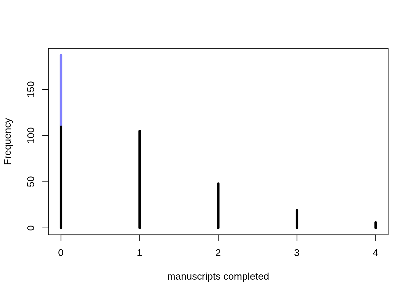

The blue part signifies the days were no manuscripts were completed because the monks were drinking. The total number of zeros is inflated, relative to a typical Poisson distribution.

To fit this Zero-Inflated Poisson model, we can use the function dzipois() provided in the Rethinking-package. The prior for the probability of drinking is nudged so that there is more mass below 0.5, the monks probably don’t drink more often than not:

ap <- rnorm(1000, -1.5, 1)
p <- inv_logit(ap)
dens(p)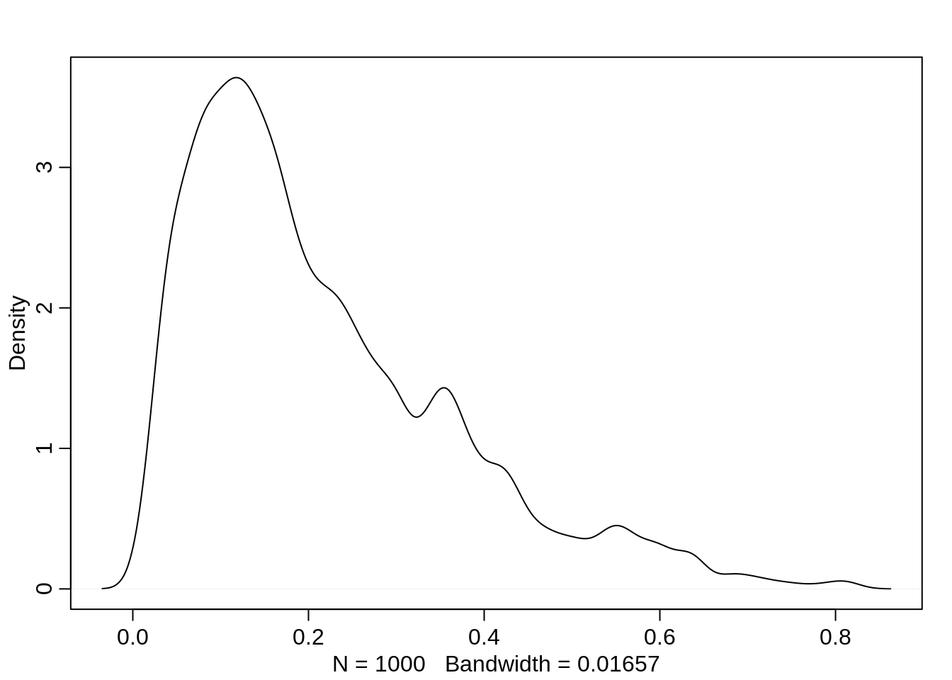

The model then looks as follows:

m12.4 <- ulam(
  alist(
    y ~ dzipois( p, lambda ),
    # p = probability monks are drinking
    logit(p) <- ap,
    # lambda = rate for completing manuscripts
    log(lambda) <- al,
    ap ~ dnorm( -1.5, 1 ),
    al ~ dnorm( 1, 0.5 )
  ), data=list(y=as.integer(y)), chains=4)

precis(m12.4)

          mean         sd       5.5%      94.5%    n_eff    Rhat4
ap -1.27943087 0.37228853 -1.9347033 -0.7735818 584.0565 1.003241
al  0.01190568 0.09243819 -0.1376475  0.1624185 649.3856 1.009246

On the natural scale, those estimates are:

inv_logit(-1.28)

[1] 0.2175502

exp(0.01)

[1] 1.01005

Note that we get a very good estimate of the proportion of days the monks drink, even though we can’t say for any particular day whether or not they drank.

The function dzipois() already does most of the work for us, but let’s check how such a model is implemented:

m12.4_alt <- ulam(
  alist(
    # log-lkhd for non-zero values: (1-p)=prob of not drinking
    # poisson_lpmf = probability of finishing y manuscripts
    y|y>0 ~ custom( log( 1-p ) + poisson_lpmf(y|lambda ) ),
    # log-lkhd for zero values: p=prob of drinking
    # (1-p)*exp(lambda) = prob of finishing zero manuscripts when not drinking
    y|y==0 ~ custom( log( p + (1-p)*exp(lambda ) )),
    logit(p) <- ap,
    log(lambda) <- al,
    ap ~ dnorm(-1.5, 1),
    al ~ dnorm(1, 0.5)
  ), data=list(y=as.integer(y)), chains=4
)

However, for numerical stability, it is better to use the functions log1m(p) for log(1-p) and log_mix(p, 0, poisson_lpmf(0|lambda)) instead of log(p + (1-p)*exp(lambda)).

m12.4_alt <- ulam(
  alist(
    # log-lkhd for non-zero values: (1-p)=prob of not drinking
    # poisson_lpmf = probability of finishing y manuscripts
    y|y>0 ~ custom( log1m( p ) + poisson_lpmf(y|lambda ) ),
    # log-lkhd for zero values: p=prob of drinking
    # (1-p)*exp(lambda) = prob of finishing zero manuscripts when not drinking
    y|y==0 ~ custom( log_mix( p, 0, poisson_lpmf(0|lambda) ) ),
    logit(p) <- ap,
    log(lambda) <- al,
    ap ~ dnorm(-1.5, 1),
    al ~ dnorm(1, 0.5)
  ), data=list(y=as.integer(y)), chains=4
)

This gives us the same estimates as m12.4:

precis(m12.4_alt)

          mean         sd       5.5%      94.5%    n_eff     Rhat4
ap -1.26899142 0.34561667 -1.8757107 -0.8064936 605.9883 1.0004240
al  0.01130696 0.08613438 -0.1257928  0.1483133 601.1485 0.9994628

It’s also helps to look at the stan code of the model:

stancode(m12.4_alt)

data{
    int y[365];
}
parameters{
    real ap;
    real al;
}
model{
    real p;
    real lambda;
    al ~ normal( 1 , 0.5 );
    ap ~ normal( -1.5 , 1 );
    lambda = al;
    lambda = exp(lambda);
    p = ap;
    p = inv_logit(p);
    for ( i in 1:365 ) 
        if ( y[i] == 0 ) target += log_mix(p, 0, poisson_lpmf(0 | lambda));
    for ( i in 1:365 ) 
        if ( y[i] > 0 ) target += log1m(p) + poisson_lpmf(y[i] | lambda);
}

The most important of the model is in the for loop, iterating over each observation. It adds the log-likelihood to the variable target which is the log posterior mass. The suffix _lpmf means it’s the log probability mass function. (For continuous variables the suffix would be _lpdf, log probability density function).