Explicit Multinomial Model

In the explicit multinomial model we need \(K-1\) linear models for \(K\) different events. In our example, we’d thus have two different linear models.

We first simulate the career choices:

library(rethinking)
set.seed(2405)
N <- 1000                # number of individuals
income <- 1:3           # expected income of each career
score <- 0.5*1:3        # scores for each career, based on income

# convert scores to probabilities
(p <- softmax(score[1], score[2], score[3]) )

[1] 0.1863237 0.3071959 0.5064804

Next, we simulate the career choice an individual made.

career <- sample(1:3, N, prob=p, replace=TRUE)

To fit the model, we use the dcategorical likelihood.

m10.16 <- map(
  alist(
    career ~ dcategorical( softmax( 0, s2, s3 )),
    s2 <- b*2,         # linear model for event type 2
    s3 <- b*3,         # linear model for event type 3
    b  ~ dnorm(0, 5)
  ), data=list(career=career)
)

precis(m10.16)

       mean         sd      5.5%     94.5%
b 0.3499246 0.02952974 0.3027303 0.3971188

So what does this estimate mean? From the parameter b we can compute the scores s2 = 0.62 and s3 = 0.93. The probabilities are then computed from these scores via softmax(). However, these score are very difficult to interpret. In this example, we assigned a fixed score of 0 to the first event, but we also could have assigned a fixed score to the second or third event. The score would be very different in that case. The probabilities obtained through softmax() will stay the same though, so it’s absolutely important to always convert these scores to probabilities.

post <- extract.samples(m10.16)
post$s2 <- post$b * 2
post$s3 <- post$b * 3
probs <- apply(post, 1, function(x) softmax(0, x[2], x[3]))
(pr <- apply(probs, 1, mean) )

[1] 0.1705797 0.3428060 0.4866143

The probabilities are reasonably close to the one we used to simulate our data.

For comparison, the proportions of our simulated data:

table(career) / length(career)

career
    1     2     3 
0.180 0.314 0.506 

Note again, the scores we obtain from the model are very different from the scores we used for the simulation, only the probabilities match!

Let’s have a look at the densities for each probability:

dens(probs[1,], main="Probability for Event 1")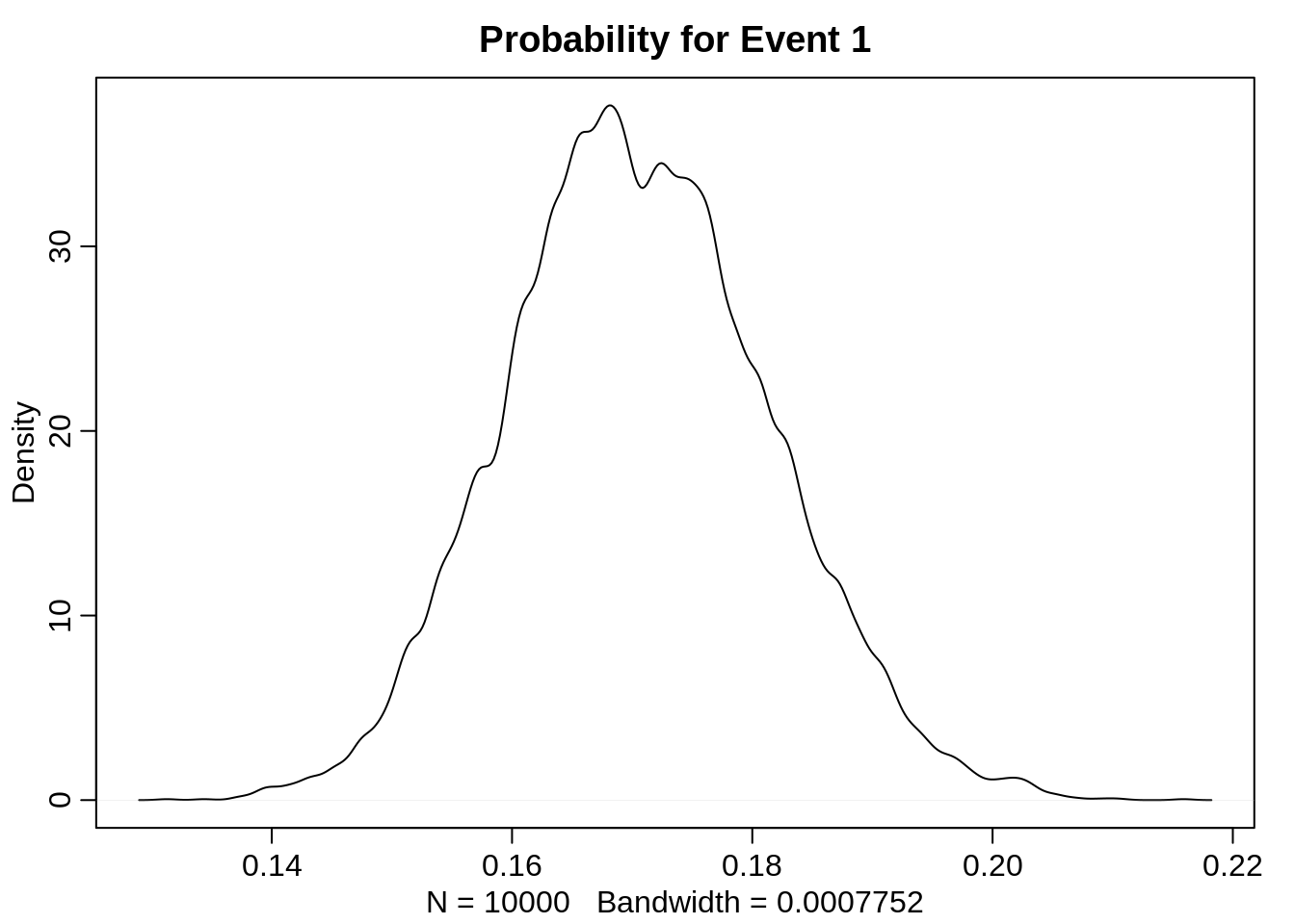

dens(probs[2,], main="Probability for Event 2")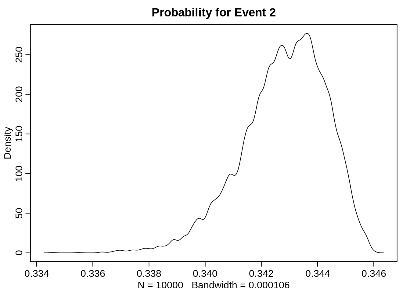

dens(probs[3,], main="Probability for Event 3")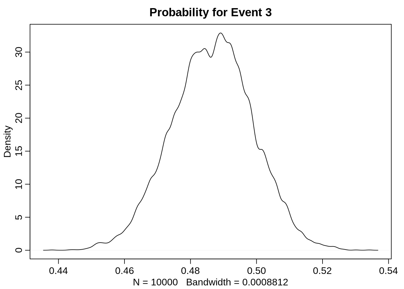

The distribution for the probability of the second event is heavily skewed. I assume this is since the three probabilities are not linearly independent of each other: They need to sum up to 1. Furthermore, we constructed the non-fixed scores as multiples of each other.

Further notes

There are various ways how to put the linear models and its scores in the softmax. Here we used

s1 <- 0
s2 <- b*2
s3 <- b*3

which translates to trying to find a \(\beta\) such that \[\begin{align*} p_1 = 0.186 &= \frac{1}{1 + \exp(2\beta) + \exp(3\beta)} + \epsilon \\ p_2 = 0.307 &= \frac{\exp(2\beta)}{1 + \exp(2\beta) + \exp(3\beta)} + \epsilon \\ p_3 = 0.506 &= \frac{\exp(3\beta)}{1 + \exp(2\beta) + \exp(3\beta)} + \epsilon . \end{align*}\] But actually, even without the error term \(\epsilon\), it’s not guaranteed that such a \(\beta\) exists. In this case, such a \(\beta\) does not exist, so the best \(\beta\) is the one that minimizes the error term. The solution to this optimization problem is indeed very close to the result we got for b.

There are also other possibilities in how we specify our model. One option for example would be to use different multiplicands for the scores:

s1 <- 0
s2 <- b
s3 <- b*2

which would indeed get better estimates in this case, since there is a \(\beta\) that almost solves the resulting equations exactly. For such a model, we would get the following estimate for \(\beta\)

       mean         sd      5.5%     94.5%
b 0.5098878 0.04125471 0.4439548 0.5758208

and the resulting probability estimates would be

[1] 0.1840538 0.3060746 0.5098716

For comparison, the proportions in our simulated data:

career
    1     2     3 
0.180 0.314 0.506 

These are quite close!

We don’t need to restrict ourselves to just one parameter for the scores and its multiples, we an also introduce another parameter for each score. For example, we could specify the models as follows:

s1 <- 0
s2 <- b2
s3 <- b2 + b3

This also gives better estimates than the original model but also introduces correlation between b2 and b3.

        mean        sd      5.5%     94.5%
b2 0.5563025 0.0934674 0.4069236 0.7056815
b3 0.4771160 0.0718306 0.3623168 0.5919151

The resulting probability estimates are

[1] 0.1800222 0.3139969 0.5059809

Interestingly, if we use a model, where each score gets its own parameter as follow

s1 <- 0
s2 <- b2
s3 <- b3

the correlation of the estimates get worse:

        mean         sd      5.5%     94.5%
b2 0.5560173 0.09345729 0.4066545 0.7053801
b3 1.0331494 0.08675576 0.8944969 1.1718018

The resulting probabilities:

[1] 0.1800629 0.3139782 0.5059589

In total, which model specification to pick in an explicit multinomial is not quite straightforward.

N <- 100
# simulate family incomes for each individual
family_income <- runif(N)
# assign a unique coefficient for each type of event
b <- (1:-1)
career <- c()
for (i in 1:N) {
  score <- 0.5*(1:3) +   b * family_income[i]
  p <- softmax(score[1], score[2], score[3])
  career[i] <- sample(1:3, size=1, prob = p)
}

m10.17 <- map(
  alist(
    career ~ dcategorical( softmax( 0, s2, s3)),
    s2 <- a2 + b2*family_income,
    s3 <- a3 + b3*family_income,
    c(a2, a3, b2, b3) ~ dnorm(0, 5)
  ), 
  data=list(career=career, family_income=family_income)
)
precis(m10.17)

         mean        sd       5.5%      94.5%
a2 -0.6593230 0.5301211 -1.5065589  0.1879128
a3  0.9576812 0.4229572  0.2817140  1.6336485
b2  1.0681466 0.8794221 -0.3373397  2.4736329
b3 -1.4571748 0.8330821 -2.7886009 -0.1257488

scores <- link(m10.17)

str(scores)

List of 2
 $ s3: num [1:1000, 1:100] 0.754 0.475 1.308 0.646 0.896 ...
 $ s2: num [1:1000, 1:100] -0.956 -0.882 -0.71 -0.935 -0.464 ...

apply(softmax(0, scores$s2[,1], scores$s3[,1]), 2, mean)

[1] 0.2655084 0.1576247 0.5768670

Multinomial using Poisson

One way to fit a multinomial likelihood is to refactor it into a series of Poisson likelihoods. It is often computationally easier to use Poisson rather than multinomial likelihood. We first will take an example from earlier with only two events (that is, a binomial case) and model it using Poisson regression:

data("UCBadmit")
d <- UCBadmit

First the binomial model for comparison:

set.seed(2405)
m_binom <- map(
  alist(
    admit ~ dbinom(applications, p),
    logit(p) <- a,
    a ~ dnorm(0, 100)
  ), data=d
)
precis(m_binom)

        mean         sd       5.5%      94.5%
a -0.4567393 0.03050707 -0.5054955 -0.4079832

And then the Poisson model. To obtain the probability of admission, we model both the rate of admission and the rate of rejection using Poisson:

d$rej <- d$reject
m_pois <- map2stan(
  alist(
    admit ~ dpois(lambda1),
    rej ~ dpois(lambda2),
    log(lambda1) <- a1,
    log(lambda2) <- a2,
    c(a1, a2) ~ dnorm(0, 100)
  ), data=d, chains=3, cores=3
)

We will consider only the posterior means.

For the binomial model, the inferred probability of admission is:

 logistic(coef(m_binom)) 

        a 
0.3877596 

In the Poisson model, the probability of admission is given by: \[\begin{align*} p_{ADMIT} = \frac{\lambda_1}{\lambda_1 + \lambda_2} = \frac{\exp(a_1)}{\exp(a_1) + \exp(a_2)} \end{align*}\] That is:

a <- as.numeric(coef(m_pois))
exp(a[1]) / ( exp(a[1]) + exp(a[2]) ) 

[1] 0.3874977

d <- data.frame(career, 
                career1= 1*(career==1), 
                career2= 1*(career==2), 
                career3= 1*(career==3))

m10.16_poisson <- map2stan(
  alist(
    career1 ~ dpois(lambda1),
    career2 ~ dpois(lambda2),
    career3 ~ dpois(lambda3),
    log(lambda1) <- b1,         # linear model for event type 1
    log(lambda2) <- b2,         # linear model for event type 2
    log(lambda3) <- b3,         # linear model for event type 3
    c(b1, b2, b3)  ~ dnorm(0, 5)
  ), data=d
)
precis(m10.16_poisson, corr = TRUE)

a <- as.numeric(coef(m10.16_poisson))
exp(a) / sum( exp(a)  )

[1] 0.2985534 0.2691924 0.4322543

career
   1    2    3 
0.30 0.27 0.43